Packages loaded globally

# Set the seed so our results are reproducible:
set.seed(2020)

# Required packages
library(tximport)
library(DESeq2)
library(Glimma)
library(vsn)

# Mouse annotation package we'll use for gene identifier conversion
library(biomaRt)

# We will need them for data handling
library(magrittr)
library(ggrepel)
library(dplyr)
library(tidyverse)
library(readr)

# plotting
library(ggplot2)
library(EnhancedVolcano)
library(ComplexUpset)
library(ComplexHeatmap)
library(RColorBrewer)

Differential expression analysis

Input data

In case our objects from part 1 are not present in the environment, here we re-load them:

dds <- readRDS(file = "./results/dds.rds")
colData <- readRDS(file = "./results/colData.rds")
txi <- readRDS(file = "./results/txi.rds")

Run `DESeq` function

The standard differential expression analysis steps in DESeq2 are wrapped into a single function, DESeq. This function performs the following key steps:

Estimation of size factors: DESeq2 calculates size factors for each sample to normalize the count data and account for differences in library size or sequencing depth.
Estimation of dispersions: DESeq2 estimates gene-wise dispersions, which model the relationship between the mean and variance of counts across samples. This accounts for the mean-variance dependency often observed in RNA-Seq data.
Fitting the negative binomial generalized linear model: DESeq2 fits a negative binomial GLM to the count data, using the design formula specified during the creation of the DESeqDataSet object.
Wald statistics: DESeq2 computes Wald statistics and p-values to test for differential expression between conditions or levels of the variables in the design formula. Note that the Wald statistic is the default test approach. DESeq2 also provides the likelihood ratio test.

In summary, DESeq2 provides a streamlined workflow for differential expression analysis, incorporating normalization, dispersion estimation, and statistical testing, while allowing users to specify the desired comparisons and extract results tailored to their experimental design

dds <- DESeq(dds)

# checking coefficient by resultsNames(dds):

resultsNames(dds)

## [1] "Intercept"                     "Condition_Transplant_vs_Naive"

# Dispersion plot

plotDispEsts(dds)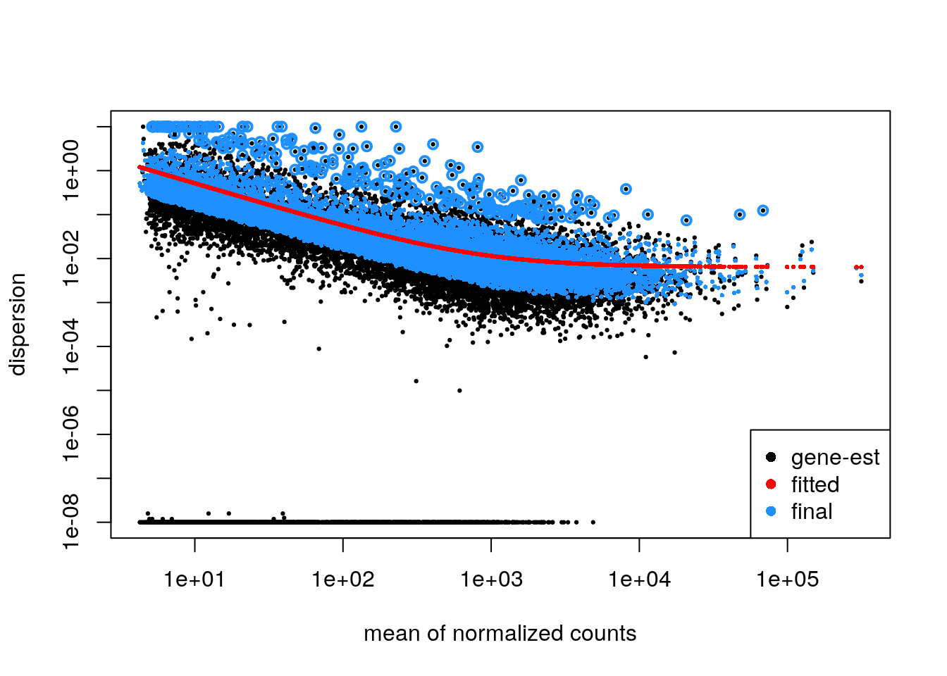

In a DESeq2 analysis, the dispersion plot visualizes the relationship between a gene’s mean expression level and its dispersion estimate. Dispersion, in this context, quantifies the degree to which the observed count data for a gene varies around its expected value under the negative binomial model.

Importance for Assumptions

The dispersion plot is a crucial diagnostic tool for assessing the validity of several key assumptions underlying the DESeq2 analysis:

Mean-Variance Relationship: DESeq2 assumes a specific relationship between a gene’s mean expression level and its variance (or dispersion). The dispersion plot helps verify whether this assumed relationship holds true in the data. Typically, genes with lower mean expression exhibit higher dispersion (more variability) than those with higher mean expression.
Model Fit: The dispersion estimates for each gene should ideally align with the fitted dispersion trend line. Substantial deviations from this trend might indicate that the negative binomial model doesn’t adequately capture the variance structure of the data.
Outliers: The dispersion plot can help identify outlier genes with unusually high dispersion estimates compared to other genes with similar mean expression levels. These outliers might warrant further investigation as they could be indicative of technical artifacts or biological phenomena not accounted for by the model.

A well-behaved dispersion plot should show:

Overall trend: A decreasing trend in dispersion as mean expression increases. Fit to the model: Most gene-wise dispersion estimates should cluster around the fitted trend line. Few outliers: A small number of points far from the trend line might indicate outliers.

By carefully examining the dispersion plot, researchers can assess whether their data conforms to the assumptions of the DESeq2 model, identify potential issues, and make informed decisions about downstream analysis steps.

`Transplant_vs_Naive` pair-wise comparision

The results function is used to extract a results table containing log2 fold changes, p-values, and adjusted p-values from the DESeq analysis. By default, the results are generated for the comparison of the last level of the last variable in the design formula against the reference level.

However, users can specify the desired comparison using the name or contrast arguments in the results function. The contrast argument allows for precise specification of the levels and order of comparison, while the name argument can be used for simple two-group comparisons. It’s important to note that DESeq2 performs independent filtering by default, which removes genes with low mean normalized counts across all samples. This step aims to improve the estimation of dispersion and reduce the multiple testing burden.

## Transplant_vs_Naive
resCondition <- results(dds, contrast = c("Condition", "Transplant", "Naive"))
summary(resCondition)

## 
## out of 15486 with nonzero total read count
## adjusted p-value < 0.1
## LFC > 0 (up)       : 3721, 24%
## LFC < 0 (down)     : 3420, 22%
## outliers [1]       : 61, 0.39%
## low counts [2]     : 0, 0%
## (mean count < 4)
## [1] see 'cooksCutoff' argument of ?results
## [2] see 'independentFiltering' argument of ?results

Shrinkage of log fold change

Shrinking log fold change (LFC) estimates is a beneficial technique to enhance the visualization and ranking of genes. To accomplish this shrinkage, we utilize the lfcShrink function for the dds object. In this example, we employ the apeglm method for effect size shrinkage (Zhu, Ibrahim, and Love 2018), which offers an improvement over the previously used estimator.

apeglm is the adaptive t prior shrinkage estimator from the apeglm package (Zhu, Ibrahim, and Love 2018). As of version 1.28.0, it is the default estimator.
ashr is the adaptive shrinkage estimator from the ashr package (Stephens 2016). Here DESeq2 uses the ashr option to fit a mixture of Normal distributions to form the prior, with method=“shrinkage”.
normal is the the original DESeq2 shrinkage estimator, an adaptive Normal distribution as prior.

#--------------- Transplant_vs_Naive: Condition_Transplant_vs_Naive --------------

dir.create("./results/Transplant_vs_Naive", recursive = TRUE)

# lfcShrink function
Transplant_vs_Naive <- lfcShrink(dds, coef="Condition_Transplant_vs_Naive", type="apeglm")

Transplant_vs_Naive

## log2 fold change (MAP): Condition Transplant vs Naive 
## Wald test p-value: Condition Transplant vs Naive 
## DataFrame with 15486 rows and 5 columns
##                         baseMean log2FoldChange     lfcSE      pvalue        padj
##                        <numeric>      <numeric> <numeric>   <numeric>   <numeric>
## ENSMUSG00000000001.5  3992.86278     0.00063763 0.0559028 9.92683e-01 9.95285e-01
## ENSMUSG00000000028.16  584.56681     2.40697733 0.1753700 5.17428e-44 3.72959e-42
## ENSMUSG00000000037.18    7.49848    -0.13626169 0.3776449 4.39381e-01 5.86031e-01
## ENSMUSG00000000056.8   366.29757     0.33061464 0.1533012 1.96559e-02 4.91078e-02
## ENSMUSG00000000058.7  2117.12191    -0.13734295 0.0768850 6.85395e-02 1.38344e-01
## ...                          ...            ...       ...         ...         ...
## ENSMUSG00002076377.1    118.0144     1.19874095  0.478207 0.000935118  0.00338278
## ENSMUSG00002076457.1     12.1973    -0.05208992  0.359533 0.761654504  0.84851370
## ENSMUSG00002076463.1     52.4421     0.29617535  0.262898 0.154408446  0.26704230
## ENSMUSG00002076763.1     18.2897    -0.00998566  0.317344 0.958042773  0.97478956
## ENSMUSG00002076916.1     48.3010     0.05373479  0.278437 0.793762229  0.86958682

Explore the `DESeq2` result

For the purposes of this workshop we will use the results which have implemented shrinkage of log2 fold changes (from the Transplant_vs_Naive variable).

P-value histogram plot

Visualizing the histogram of p-values is a valuable practice when assessing the distribution of your hypotheses (null vs alternative). This plot aids in evaluating whether your data meets the assumptions required for False Discovery Rate (FDR) correction. Although FDR correction is typically applied to control for false positives, there are specific instances where careful consideration is warranted.

These edge cases go beyond the scope of this workshop, but we encourage trainees to read the following post that nicely summarize data patterns to be aware of: http://varianceexplained.org/statistics/interpreting-pvalue-histogram/

# distribution of p-vals (always want to plot non-corrected p-values for this)
hist(Transplant_vs_Naive$pvalue)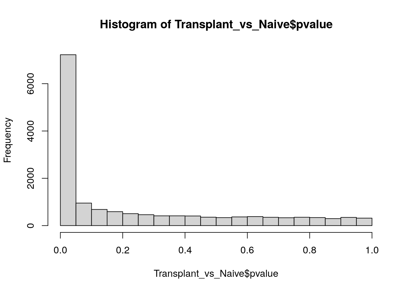

Each bar represents the number of genes with a p-value in the given bin (bin size=0.05).

MA Plot

We can visualize the results in many ways. A good check is to explore the relationship between log2fold changes, significant DE genes and the genes mean count. DESeq2 provides a useful function to do so, plotMA().

plotMA(Transplant_vs_Naive)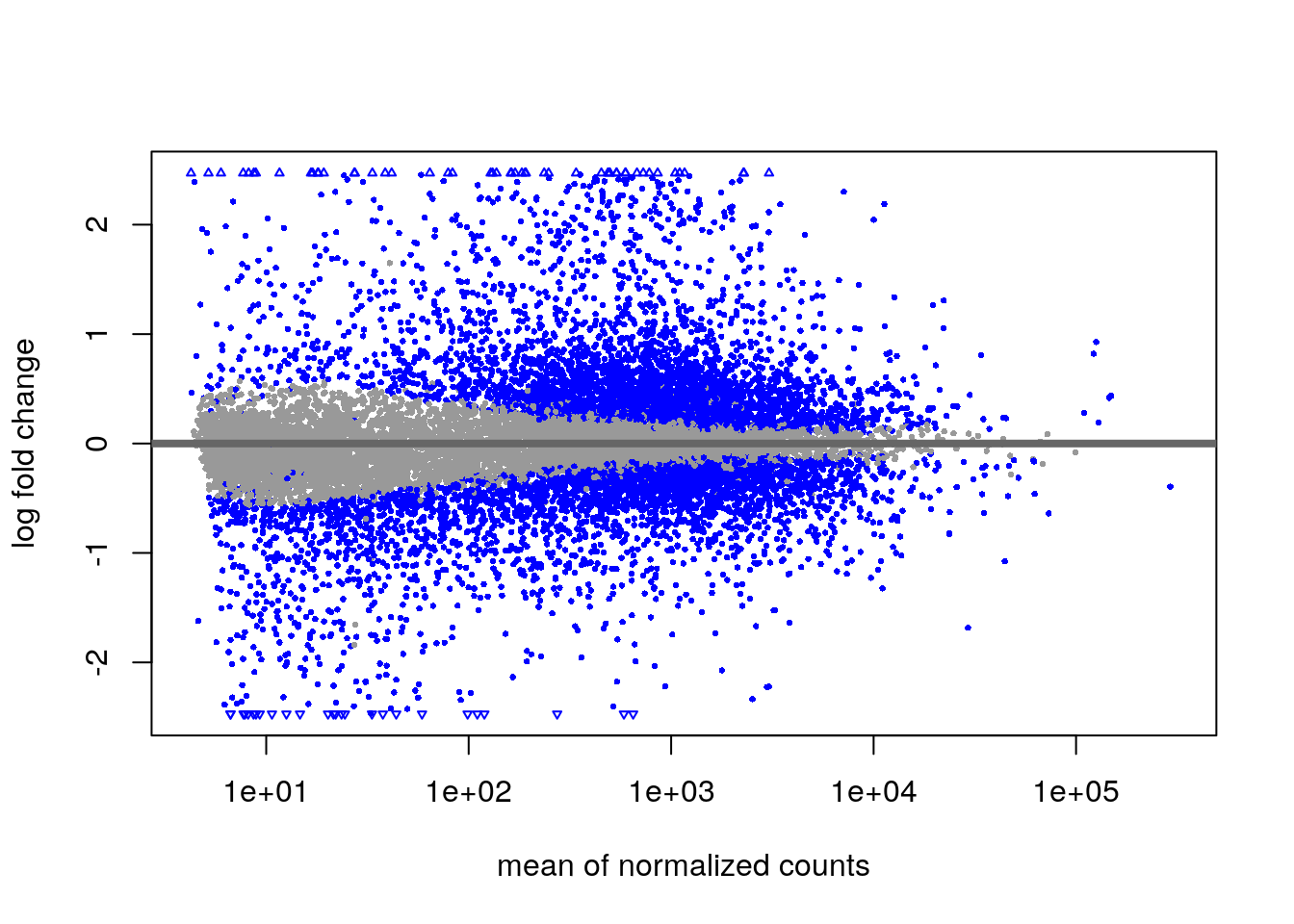

Summary statistics

In DESeq2, the adjusted p-value (also known as padj) is a modified version of the raw p-value that accounts for multiple hypothesis testing. When you perform thousands of statistical tests simultaneously (as in differential gene expression analysis), the probability of observing some false positives increases. The adjusted p-value controls for this by estimating the false discovery rate (FDR). The Default cutoff is adjusted p-value < 0.1.

Discussion Question

In part 1, we applied pre-filtering to remove very low abundance genes. How is pre-filtering linked to multiple hypothesis testing / false discovery rates?

Default FDR Correction Method

The default method for FDR correction in DESeq2 is the Benjamini-Hochberg (BH) procedure. This method ranks the p-values from smallest to largest and calculates an adjusted p-value for each gene based on its rank and the total number of tests performed. The adjusted p-value represents the estimated proportion of false positives among all genes with an equal or smaller p-value.

summary(Transplant_vs_Naive)

## 
## out of 15486 with nonzero total read count
## adjusted p-value < 0.1
## LFC > 0 (up)       : 3721, 24%
## LFC < 0 (down)     : 3420, 22%
## outliers [1]       : 61, 0.39%
## low counts [2]     : 0, 0%
## (mean count < 4)
## [1] see 'cooksCutoff' argument of ?results
## [2] see 'independentFiltering' argument of ?results

You can customize adjusted p-value cutoff by changing the default parameter:

summary(Transplant_vs_Naive, alpha = 0.05)

## 
## out of 15486 with nonzero total read count
## adjusted p-value < 0.05
## LFC > 0 (up)       : 3342, 22%
## LFC < 0 (down)     : 2854, 18%
## outliers [1]       : 61, 0.39%
## low counts [2]     : 0, 0%
## (mean count < 4)
## [1] see 'cooksCutoff' argument of ?results
## [2] see 'independentFiltering' argument of ?results

At a first glance, this data suggests that there are significantly large transcriptomics alterations based on adjusted p-value < 0.05.

Challenge: different approaches to limit the DEGs count

Click here for solution

summary(Transplant_vs_Naive, alpha = 0.01)

## 
## out of 15486 with nonzero total read count
## adjusted p-value < 0.01
## LFC > 0 (up)       : 2730, 18%
## LFC < 0 (down)     : 2134, 14%
## outliers [1]       : 61, 0.39%
## low counts [2]     : 0, 0%
## (mean count < 4)
## [1] see 'cooksCutoff' argument of ?results
## [2] see 'independentFiltering' argument of ?results

Note: the summary function is simplistic in nature. In the later portions of the workshop we will also cover another variable to filter results on: log2 fold changes.

Sort by Adjusted p.value

Transplant_vs_Naive <- Transplant_vs_Naive[order(Transplant_vs_Naive$padj),]

head(Transplant_vs_Naive)

## log2 fold change (MAP): Condition Transplant vs Naive 
## Wald test p-value: Condition Transplant vs Naive 
## DataFrame with 6 rows and 5 columns
##                        baseMean log2FoldChange     lfcSE       pvalue         padj
##                       <numeric>      <numeric> <numeric>    <numeric>    <numeric>
## ENSMUSG00000020649.12   3044.32        2.64171 0.0792717 1.64953e-244 2.54441e-240
## ENSMUSG00000040204.7    2289.67        3.06535 0.1037299 4.37636e-193 3.37526e-189
## ENSMUSG00000027342.15   6740.49        1.49248 0.0515139 1.42499e-185 7.32684e-182
## ENSMUSG00000020914.18   7125.77        2.30101 0.0856891 5.38773e-160 2.07764e-156
## ENSMUSG00000005470.9    1164.67        2.47450 0.0951897 5.21848e-150 1.60990e-146
## ENSMUSG00000006678.7    1092.42        1.78528 0.0687794 1.26120e-149 3.24234e-146

Make annotation object

At this point, we will create an annotation object which we will use in the later section of this workshop to add annotation information (e.g.: gene names) to our results.

Note that in the code below we select mm39 (GENCODE release M32) corresponding to Ensembl 109 since this is the genome / GTF versions we used in secondary analysis. You should always aim to match the genomic version in tertiary analysis to what was used in the secondary analysis.

Also note that while there are many ways to annotate your data, the code chunks below implements functions from the biomaRt package to fetch the annotations.

As a starting point, let’s check the available Ensembl versions, to ensure we select the correct one for our data:

# check available urls (current and archives):
listEnsemblArchives()

##              name     date                                 url version current_release
## 1  Ensembl GRCh37 Feb 2014          https://grch37.ensembl.org  GRCh37                
## 2     Ensembl 112 May 2024 https://may2024.archive.ensembl.org     112               *
## 3     Ensembl 111 Jan 2024 https://jan2024.archive.ensembl.org     111                
## 4     Ensembl 110 Jul 2023 https://jul2023.archive.ensembl.org     110                
## 5     Ensembl 109 Feb 2023 https://feb2023.archive.ensembl.org     109                
## 6     Ensembl 108 Oct 2022 https://oct2022.archive.ensembl.org     108                
## 7     Ensembl 107 Jul 2022 https://jul2022.archive.ensembl.org     107                
## 8     Ensembl 106 Apr 2022 https://apr2022.archive.ensembl.org     106                
## 9     Ensembl 105 Dec 2021 https://dec2021.archive.ensembl.org     105                
## 10    Ensembl 104 May 2021 https://may2021.archive.ensembl.org     104                
## 11    Ensembl 103 Feb 2021 https://feb2021.archive.ensembl.org     103                
## 12    Ensembl 102 Nov 2020 https://nov2020.archive.ensembl.org     102                
## 13    Ensembl 101 Aug 2020 https://aug2020.archive.ensembl.org     101                
## 14    Ensembl 100 Apr 2020 https://apr2020.archive.ensembl.org     100                
## 15     Ensembl 99 Jan 2020 https://jan2020.archive.ensembl.org      99                
## 16     Ensembl 98 Sep 2019 https://sep2019.archive.ensembl.org      98                
## 17     Ensembl 97 Jul 2019 https://jul2019.archive.ensembl.org      97                
## 18     Ensembl 80 May 2015 https://may2015.archive.ensembl.org      80                
## 19     Ensembl 77 Oct 2014 https://oct2014.archive.ensembl.org      77                
## 20     Ensembl 75 Feb 2014 https://feb2014.archive.ensembl.org      75                
## 21     Ensembl 54 May 2009 https://may2009.archive.ensembl.org      54

We can see from the output above, that the url matching the Ensembl 109 version is https://feb2023.archive.ensembl.org. Thus, we set the hosting url below to this specific version.

Further, biomaRt provides several attributes you may add to your data for annotation. The attributes selected below are some of the most commonly used and needed metadata:

You can list all available attributes for a glance listAttributes(ensembl) where ensembl is the Mart object we will create in this section.

# Specify the version specific archive:
host_url <- "https://feb2023.archive.ensembl.org"

# attributes
attributes_to_add <- c("ensembl_gene_id", "external_gene_name","gene_biotype",
                       "description","chromosome_name","start_position",
                       "end_position","strand")

Next, select the species. If you are unsure on how to properly add your species, you can see the options by running listDatasets(mart=useMart("ENSEMBL_MART_ENSEMBL", host = host_url))

species <- "mmusculus_gene_ensembl"

With all required parameters set for biomaRt, run the code chunk below to: * Connect to the selected BioMart database * Use Ensembl IDs as the input query * Fetch the annotation information

ensembl <- useMart("ENSEMBL_MART_ENSEMBL", dataset = species, host = host_url)

listMarts(host=host_url)

##                biomart                version
## 1 ENSEMBL_MART_ENSEMBL      Ensembl Genes 109
## 2   ENSEMBL_MART_MOUSE      Mouse strains 109
## 3     ENSEMBL_MART_SNP  Ensembl Variation 109
## 4 ENSEMBL_MART_FUNCGEN Ensembl Regulation 109

# although we filtered counts initially, we
# fetch the annotation for all genes:
gene_ids <- rownames(txi$counts)

# remove GENCODE gene version to make ids compatible to Ensemvbl:
gene_ids <- gsub("\\.[0-9]+","",gene_ids) 

head(gene_ids)

## [1] "ENSMUSG00000000001" "ENSMUSG00000000003" "ENSMUSG00000000028" "ENSMUSG00000000031" "ENSMUSG00000000037" "ENSMUSG00000000049"

# fetch annotations
genemap <- getBM(attributes = attributes_to_add,
                 filters = "ensembl_gene_id",
                 values = gene_ids,
                 mart = ensembl,
                 useCache = FALSE)

## Batch submitting query [======>-------------------------------------------------------------------------------] 8% eta: 14sBatch
## submitting query [=============>------------------------------------------------------------------------] 17% eta: 11sBatch submitting
## query [=====================>----------------------------------------------------------------] 25% eta: 9sBatch submitting query
## [============================>---------------------------------------------------------] 33% eta: 8sBatch submitting query
## [===================================>--------------------------------------------------] 42% eta: 7sBatch submitting query
## [==========================================>-------------------------------------------] 50% eta: 6sBatch submitting query
## [=================================================>------------------------------------] 58% eta: 5sBatch submitting query
## [========================================================>-----------------------------] 67% eta: 4sBatch submitting query
## [===============================================================>----------------------] 75% eta: 3sBatch submitting query
## [=======================================================================>--------------] 83% eta: 2sBatch submitting query
## [==============================================================================>-------] 92% eta: 1s

head(genemap)

##      ensembl_gene_id external_gene_name   gene_biotype
## 1 ENSMUSG00000000001              Gnai3 protein_coding
## 2 ENSMUSG00000000003               Pbsn protein_coding
## 3 ENSMUSG00000000028              Cdc45 protein_coding
## 4 ENSMUSG00000000031                H19         lncRNA
## 5 ENSMUSG00000000037              Scml2 protein_coding
## 6 ENSMUSG00000000049               Apoh protein_coding
##                                                                                            description chromosome_name start_position
## 1 guanine nucleotide binding protein (G protein), alpha inhibiting 3 [Source:MGI Symbol;Acc:MGI:95773]               3      108014596
## 2                                                         probasin [Source:MGI Symbol;Acc:MGI:1860484]               X       76881507
## 3                                           cell division cycle 45 [Source:MGI Symbol;Acc:MGI:1338073]              16       18599197
## 4                     H19, imprinted maternally expressed transcript [Source:MGI Symbol;Acc:MGI:95891]               7      142129262
## 5                                Scm polycomb group protein like 2 [Source:MGI Symbol;Acc:MGI:1340042]               X      159865521
## 6                                                   apolipoprotein H [Source:MGI Symbol;Acc:MGI:88058]              11      108234180
##   end_position strand
## 1    108053462     -1
## 2     76897229     -1
## 3     18630737     -1
## 4    142131886     -1
## 5    160041209      1
## 6    108305222      1

nrow(genemap)

## [1] 55891

length(gene_ids) == nrow(genemap)

## [1] TRUE

saveRDS(genemap, file = "./results/genemap.rds")

Add annotation to DEG results

Now that we have the differentially expressed genes (DEG), we can use the annotated object created earlier, to add gene metadata to the DEG results:

# add the current gene_ids to new columns and remove the GENCODE version
# Note we add 2 columns (one with GENCODE version and one without it) to preserve
# version information if needed:

Transplant_vs_Naive$ensembl_gene_id_version <- rownames(Transplant_vs_Naive)
Transplant_vs_Naive$ensembl_gene_id <- rownames(Transplant_vs_Naive)

Transplant_vs_Naive$ensembl_gene_id  <- gsub("\\.[0-9]+", "", Transplant_vs_Naive$ensembl_gene_id)

# join the DEG list and biomaRt list by "ensembl_gene_id"
Transplant_vs_Naive_annotated <- dplyr::left_join(x = as.data.frame(Transplant_vs_Naive),
                                                  y = genemap,
                                                  by = (c("ensembl_gene_id")))

# add Ensembl IDs as row names:
rownames(Transplant_vs_Naive_annotated) <- Transplant_vs_Naive_annotated$ensembl_gene_id
head(Transplant_vs_Naive_annotated, 5)

##                    baseMean log2FoldChange      lfcSE        pvalue          padj ensembl_gene_id_version    ensembl_gene_id
## ENSMUSG00000020649 3044.320       2.641712 0.07927173 1.649533e-244 2.544405e-240   ENSMUSG00000020649.12 ENSMUSG00000020649
## ENSMUSG00000040204 2289.666       3.065352 0.10372992 4.376356e-193 3.375265e-189    ENSMUSG00000040204.7 ENSMUSG00000040204
## ENSMUSG00000027342 6740.487       1.492478 0.05151393 1.424992e-185 7.326835e-182   ENSMUSG00000027342.15 ENSMUSG00000027342
## ENSMUSG00000020914 7125.770       2.301005 0.08568914 5.387733e-160 2.077644e-156   ENSMUSG00000020914.18 ENSMUSG00000020914
## ENSMUSG00000005470 1164.674       2.474504 0.09518970 5.218481e-150 1.609901e-146    ENSMUSG00000005470.9 ENSMUSG00000005470
##                    external_gene_name   gene_biotype                                                                      description
## ENSMUSG00000020649               Rrm2 protein_coding                    ribonucleotide reductase M2 [Source:MGI Symbol;Acc:MGI:98181]
## ENSMUSG00000040204              Pclaf protein_coding                 PCNA clamp associated factor [Source:MGI Symbol;Acc:MGI:1915276]
## ENSMUSG00000027342               Pcna protein_coding             proliferating cell nuclear antigen [Source:MGI Symbol;Acc:MGI:97503]
## ENSMUSG00000020914              Top2a protein_coding                   topoisomerase (DNA) II alpha [Source:MGI Symbol;Acc:MGI:98790]
## ENSMUSG00000005470              Asf1b protein_coding anti-silencing function 1B histone chaperone [Source:MGI Symbol;Acc:MGI:1914179]
##                    chromosome_name start_position end_position strand
## ENSMUSG00000020649              12       24758240     24764145      1
## ENSMUSG00000040204               9       65797519     65810548      1
## ENSMUSG00000027342               2      132091082    132095234     -1
## ENSMUSG00000020914              11       98883769     98915015     -1
## ENSMUSG00000005470               8       84682136     84696826      1

Save data outputs

First, let’s save our annotated DEG list as csv file:

write.csv(Transplant_vs_Naive_annotated, 
          file = "./results/Transplant_vs_Naive/Transplant_vs_Naive_annotated_DEGlist.csv")

Second, let’s save the normalized counts as a csv file. This is critical output for data visualization as it contain normalized counts per sample:

# add normalized counts to a new vector:
normalized_counts <- as.data.frame(counts(dds, normalized = TRUE))

# add annotation
# NOTE: here we add a new column names using the `mutate` function
# as an alternative to the approach shown in the DEG results
normalized_counts_annotated <- normalized_counts %>% 
  mutate(ensembl_gene_id_version = rownames(normalized_counts),
         ensembl_gene_id = rownames(normalized_counts)) %>%
  mutate(ensembl_gene_id = gsub("\\.[0-9]+","",ensembl_gene_id)) %>%
  dplyr::left_join(x = ., y = genemap, by = (c("ensembl_gene_id")))

write.csv(normalized_counts_annotated,
          file="./results/Transplant_vs_Naive/normalized_counts.csv",
          row.names = FALSE)

To simplify the code sections below, we rename the longer variable names to shorter ones: (we explicitly named them longer in earlier sections for clarity in the workflow for teaching purposes)

T_vs_N_annotated <- Transplant_vs_Naive_annotated
counts_annotated <- normalized_counts_annotated

DEG plots

In the sections below, note that we apply an absolute log2 fold change cut-off in addition to adjusted p-values to define DEGs.

Volcano plot

EnhancedVolcano(T_vs_N_annotated,
                lab = T_vs_N_annotated$external_gene_name,
                x = "log2FoldChange",
                y = "padj",
                title = "Transplant_vs_Naive",
                pCutoff = 0.05,
                FCcutoff = 1.0,
                pointSize = 1.0,
                labSize = 4)

Visualize selected set of genes

Apply standard DEG filters adj.P.Val <= 0.05, logFC <= -1 | logFC >= 1.

T_vs_N_annotated_DEGs <- T_vs_N_annotated %>%
  dplyr::filter(padj <= 0.05, log2FoldChange <= -1 | log2FoldChange >= 1) %>%
  dplyr::arrange(dplyr::desc(abs(log2FoldChange))) %>%
  # Filter out the duplicated rows using `dplyr::distinct()`
  dplyr::distinct(external_gene_name, .keep_all = TRUE)

# Get all DE genes
genes <- T_vs_N_annotated_DEGs[order(T_vs_N_annotated_DEGs$padj), ] %>%
         rownames()

heatmapData <- normalized_counts[genes, ]

# Scale counts for visualization
heatmapData <- t(scale(t(heatmapData)))

# Add annotation
heatmapColAnnot <- data.frame(colData(dds)[, "Condition"])
heatmapColAnnot <- HeatmapAnnotation(df = heatmapColAnnot)


# Plot as heatmap
DEG_heatmap <- ComplexHeatmap::Heatmap(heatmapData,
                                       top_annotation = heatmapColAnnot,
                                       cluster_rows = TRUE, 
                                       cluster_columns = TRUE,
                                       show_row_names = FALSE)

DEG_heatmap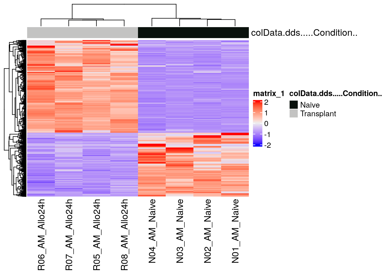

Challenge: Plot top 10 DEGs by both direction

Click here for solution

# Get top 20 DE genes
# Select top 10 up-regulated genes
top_up_genes <- T_vs_N_annotated_DEGs[order(T_vs_N_annotated_DEGs$padj), ] %>%
  filter(log2FoldChange > 1) %>%           # Focus on up-regulated (positive log2fc)
  head(20) %>%
  rownames()

# Select top 10 down-regulated genes
top_down_genes <- T_vs_N_annotated_DEGs[order(T_vs_N_annotated_DEGs$padj), ] %>%
  filter(log2FoldChange < -1) %>%           # Focus on up-regulated (negative log2fc)
  head(20) %>%
  rownames()

genes <- c(top_up_genes, top_down_genes)

heatmapData <- normalized_counts[genes, ]

# Scale counts for visualization
heatmapData <- t(scale(t(heatmapData)))

# Add annotation
heatmapColAnnot <- data.frame(colData(dds)[, "Condition"])
heatmapColAnnot <- HeatmapAnnotation(df = heatmapColAnnot)


# Plot as heatmap
DEG_heatmap <- ComplexHeatmap::Heatmap(heatmapData,
                        top_annotation = heatmapColAnnot,
                        cluster_rows = TRUE, 
                        cluster_columns = TRUE,
                        show_row_names = TRUE)

DEG_heatmap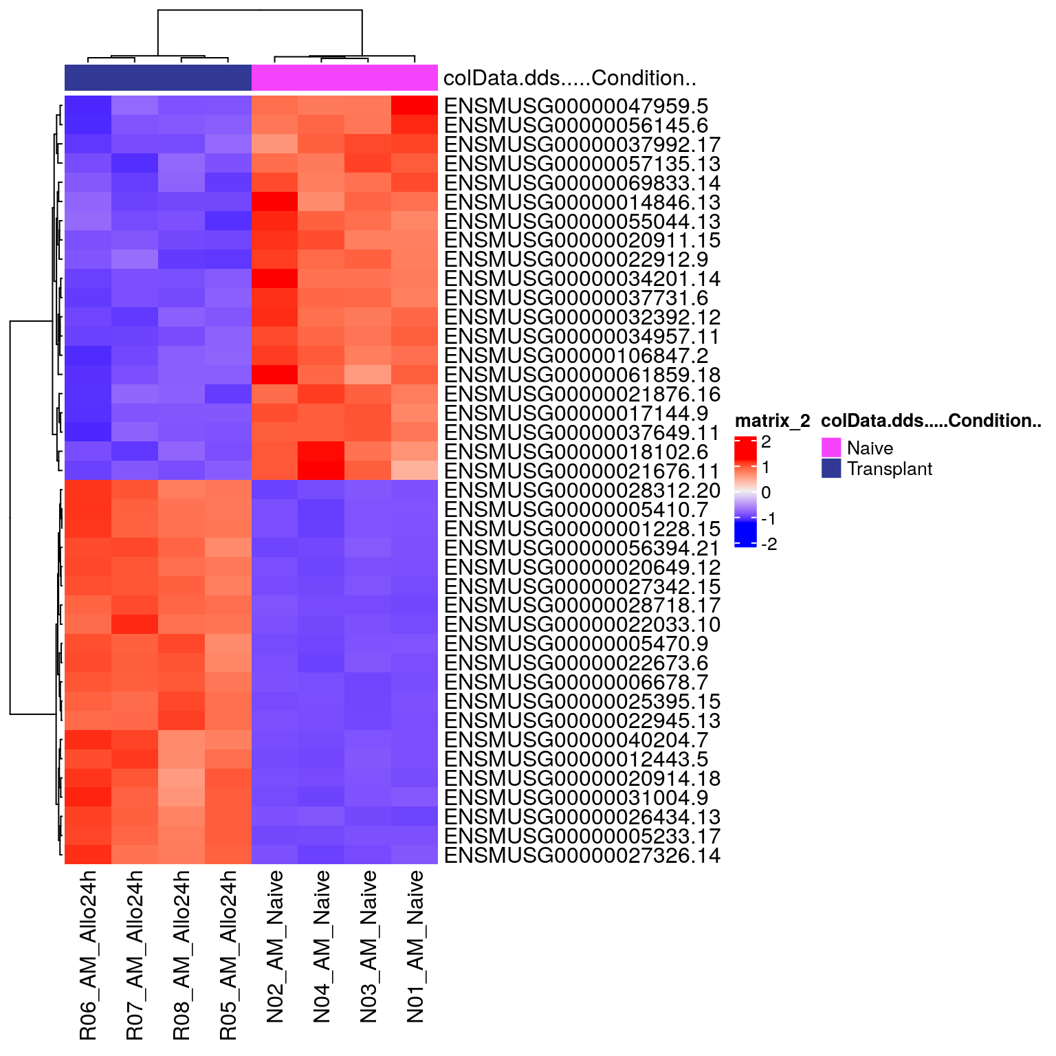

Challenge: Plot top 10 DEGs by gene names

Click here for solution

T_vs_N_fil <- T_vs_N_annotated[! is.na(T_vs_N_annotated$external_gene_name)
                               & T_vs_N_annotated$external_gene_name !="", ]

counts_fil <- counts_annotated[! is.na(counts_annotated$external_gene_name)
                               & counts_annotated$external_gene_name !="", ]

unique_gene_names <- make.unique(T_vs_N_fil$external_gene_name, sep = ".")

unique_gene_names_count <- make.unique(counts_fil$external_gene_name, sep = ".")

rownames(T_vs_N_fil) <- unique_gene_names

rownames(counts_fil) <- unique_gene_names_count

# Get top 10 DE genes
genes <- T_vs_N_fil[order(T_vs_N_fil$padj), ] %>%
         head(10) %>%
         rownames()

heatmapData <- counts_fil[genes, ]

# Scale counts for visualization
heatmapData <- t(scale(t(heatmapData[, 1:8])))

# Add annotation
heatmapColAnnot <- data.frame(colData(dds)[, "Condition"])
heatmapColAnnot <- HeatmapAnnotation(df = heatmapColAnnot)


# Plot as heatmap
DEG_heatmap <- ComplexHeatmap::Heatmap(heatmapData,
                                       top_annotation = heatmapColAnnot,
                                       cluster_rows = TRUE, 
                                       cluster_columns = TRUE,
                                       show_row_names = TRUE)

DEG_heatmap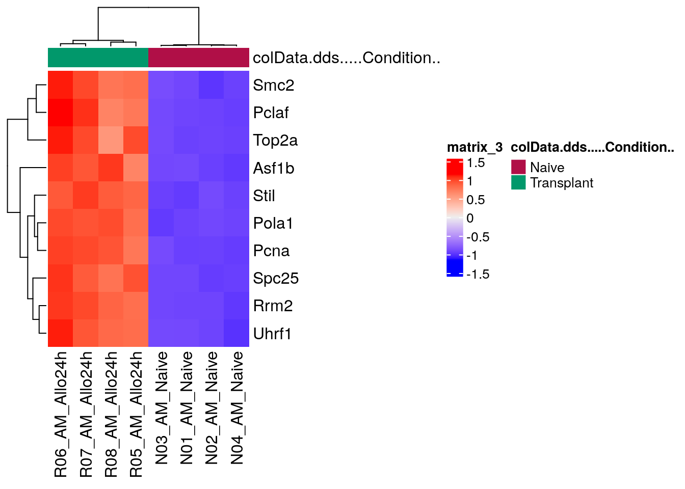

Plot selected genes

Box plot

# Define the genes of interest.
goi <- T_vs_N_fil[order(T_vs_N_fil$padj), ] %>%
  head(10) %>%
  rownames()

countData <- counts_fil[goi, 1:8]

tcounts <- t(countData) %>%
  merge(colData(dds), ., by="row.names") %>%
  gather(gene, expression, (ncol(.)-length(goi)+1):ncol(.))

Now, create a single faceted plot.

ggplot(tcounts, aes(Condition, expression, fill=Time)) + 
  geom_boxplot() + 
  facet_wrap(~gene, scales="free_y") + 
  labs(x="Condition", 
       y="Expression (log normalized counts)", 
       fill="(Time)", 
       title="Top Results")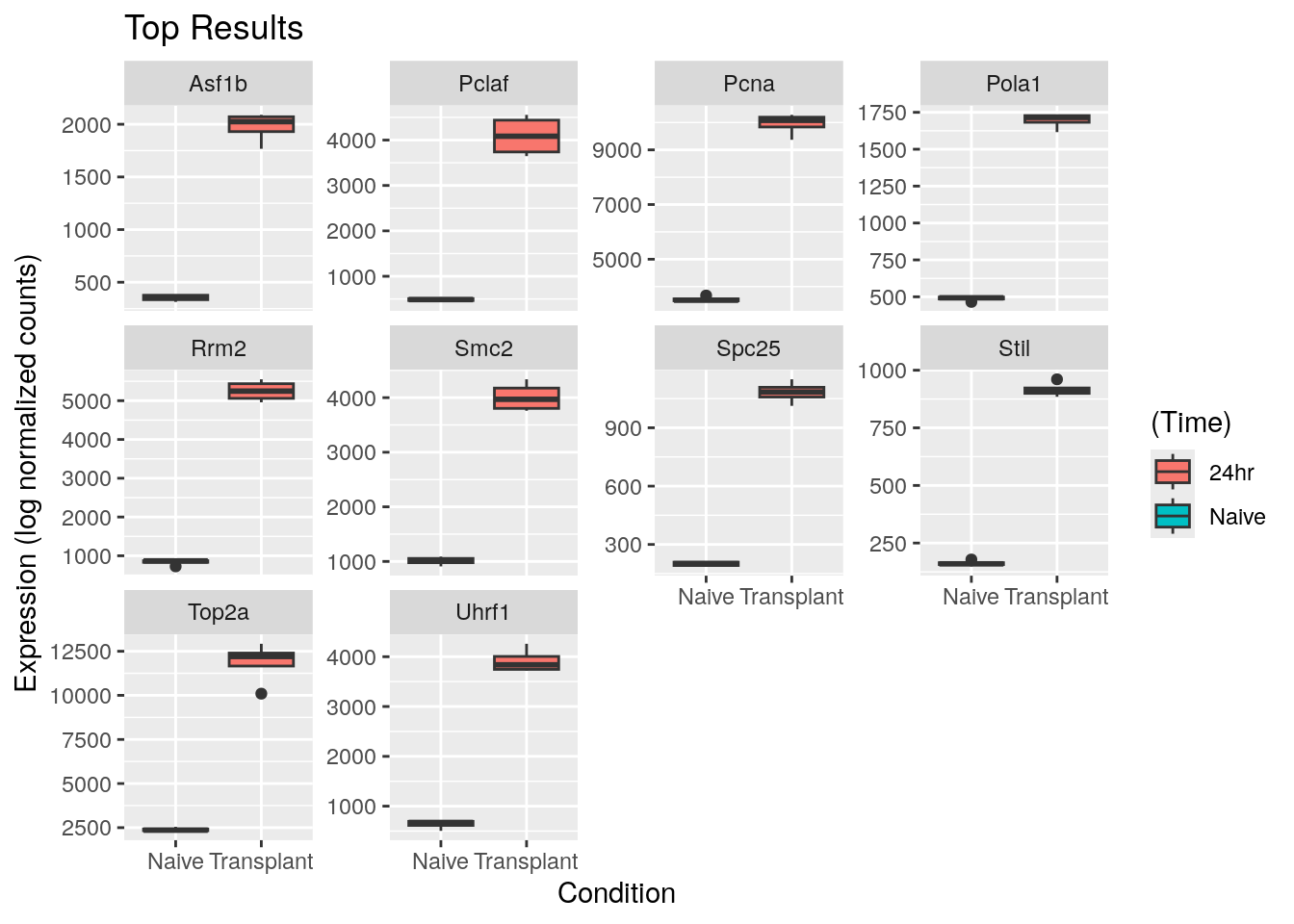

count plot

DESeq2 provides a simple count function which can be implemented for brief / quick visualizations:

plotCounts(dds, 
           gene = "ENSMUSG00000040204.7", 
           intgroup = "Condition",
           normalized = TRUE)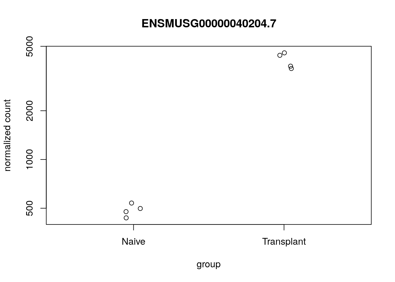

Glimma report

Glimma is an interactive R widget for creating plots for differential expression analysis, created using the Vega and htmlwidgets frameworks. The created plots can be embedded in R Markdown, or exported as standalone HTML documents.

MA Plot

The MA plot is a visualization that plots the log-fold-change between experimental groups (M) against the mean expression across all the samples (A) for each gene.

The Glimma MA plot contains two main components:

a plot of summary statistics across all genes that have been tested, and
a plot of gene expression from individual samples for a given gene

The second plot shows gene expression from the last selected sample, which can be selected from the table or directly from the summary plot.

# first choose selected annotation to be present in report
# (we choose a subset to make visualization easier/reduce # of cols)
selected_annotation <- data.frame(GeneID = rownames(normalized_counts))

selected_annotation %>% 
    mutate(ensembl_gene_id = selected_annotation$GeneID) %>%
    mutate(ensembl_gene_id = gsub("\\.[0-9]+","",ensembl_gene_id)) %>%
    plyr::join(., genemap, by = c("ensembl_gene_id")) %>%
    dplyr::select(GeneID, external_gene_name, gene_biotype) %>%
    {.} -> selected_annotation

head(selected_annotation)

##                  GeneID external_gene_name   gene_biotype
## 1  ENSMUSG00000000001.5              Gnai3 protein_coding
## 2 ENSMUSG00000000028.16              Cdc45 protein_coding
## 3 ENSMUSG00000000037.18              Scml2 protein_coding
## 4  ENSMUSG00000000056.8               Narf protein_coding
## 5  ENSMUSG00000000058.7               Cav2 protein_coding
## 6  ENSMUSG00000000078.8               Klf6 protein_coding

# use the original DESeq2 res. obj since row order is the same across all to facilitate
# NOTE: basemean are shown in the natural log scale in the report

file_name <- paste0("./results/Transplant_vs_Naive/Glimma_ma_plot.html")
    
rownames(Transplant_vs_Naive) <- Transplant_vs_Naive$ensembl_gene_id_version

Transplant_vs_Naive <- Transplant_vs_Naive[order(Transplant_vs_Naive$ensembl_gene_id_version, decreasing = FALSE),]
 
print(all(rownames(Transplant_vs_Naive) == rownames(normalized_counts))) # must always be true for glimma reports

## [1] TRUE

# select sig (arbitrary choice of padj < 0.05) - to be highlighted in MA plot
    
sig_genes <- as.numeric(Transplant_vs_Naive$padj<0.05)
    
glMDPlot(Transplant_vs_Naive, 
             status=sig_genes, 
             counts=normalized_counts,
             side.main="GeneID",
             groups=colData$Condition,
             folder = file_name,
             html = "MA-Plot",
             anno = selected_annotation,
             side.xlab = "Group",
             side.log = FALSE,
             launch=FALSE)

session info

sessionInfo()

## R version 4.3.3 (2024-02-29)
## Platform: x86_64-pc-linux-gnu (64-bit)
## Running under: Ubuntu 22.04.4 LTS
## 
## Matrix products: default
## BLAS:   /usr/lib/x86_64-linux-gnu/openblas-pthread/libblas.so.3 
## LAPACK: /usr/lib/x86_64-linux-gnu/openblas-pthread/libopenblasp-r0.3.20.so;  LAPACK version 3.10.0
## 
## locale:
##  [1] LC_CTYPE=en_US.UTF-8       LC_NUMERIC=C               LC_TIME=en_US.UTF-8        LC_COLLATE=en_US.UTF-8    
##  [5] LC_MONETARY=en_US.UTF-8    LC_MESSAGES=en_US.UTF-8    LC_PAPER=en_US.UTF-8       LC_NAME=C                 
##  [9] LC_ADDRESS=C               LC_TELEPHONE=C             LC_MEASUREMENT=en_US.UTF-8 LC_IDENTIFICATION=C       
## 
## time zone: Etc/UTC
## tzcode source: system (glibc)
## 
## attached base packages:
## [1] grid      stats4    stats     graphics  grDevices utils     datasets  methods   base     
## 
## other attached packages:
##  [1] ComplexUpset_1.3.3          EnhancedVolcano_1.20.0      RColorBrewer_1.1-3          ComplexHeatmap_2.18.0      
##  [5] lubridate_1.9.3             forcats_1.0.0               stringr_1.5.1               purrr_1.0.2                
##  [9] readr_2.1.5                 tidyr_1.3.1                 tibble_3.2.1                tidyverse_2.0.0            
## [13] dplyr_1.1.4                 ggrepel_0.9.5               ggplot2_3.5.0               magrittr_2.0.3             
## [17] biomaRt_2.58.2              vsn_3.70.0                  Glimma_2.12.0               DESeq2_1.42.1              
## [21] SummarizedExperiment_1.32.0 Biobase_2.62.0              MatrixGenerics_1.14.0       matrixStats_1.3.0          
## [25] GenomicRanges_1.54.1        GenomeInfoDb_1.38.8         IRanges_2.36.0              S4Vectors_0.40.2           
## [29] BiocGenerics_0.48.1         tximport_1.30.0            
## 
## loaded via a namespace (and not attached):
##   [1] rstudioapi_0.16.0       jsonlite_1.8.8          shape_1.4.6.1           farver_2.1.1            rmarkdown_2.26         
##   [6] GlobalOptions_0.1.2     zlibbioc_1.48.2         vctrs_0.6.5             memoise_2.0.1           RCurl_1.98-1.14        
##  [11] htmltools_0.5.8.1       S4Arrays_1.2.1          progress_1.2.3          curl_5.2.1              SparseArray_1.2.4      
##  [16] sass_0.4.9              bslib_0.7.0             htmlwidgets_1.6.4       fontawesome_0.5.2       plyr_1.8.9             
##  [21] cachem_1.0.8            lifecycle_1.0.4         iterators_1.0.14        pkgconfig_2.0.3         Matrix_1.6-5           
##  [26] R6_2.5.1                fastmap_1.1.1           GenomeInfoDbData_1.2.11 clue_0.3-65             numDeriv_2016.8-1.1    
##  [31] digest_0.6.35           colorspace_2.1-0        patchwork_1.2.0         AnnotationDbi_1.64.1    RSQLite_2.3.6          
##  [36] filelock_1.0.3          labeling_0.4.3          fansi_1.0.6             timechange_0.3.0        httr_1.4.7             
##  [41] abind_1.4-5             compiler_4.3.3          bit64_4.0.5             withr_3.0.0             doParallel_1.0.17      
##  [46] BiocParallel_1.36.0     DBI_1.2.2               hexbin_1.28.3           highr_0.10              MASS_7.3-60.0.1        
##  [51] rappdirs_0.3.3          DelayedArray_0.28.0     rjson_0.2.21            tools_4.3.3             glue_1.7.0             
##  [56] cluster_2.1.6           generics_0.1.3          gtable_0.3.5            tzdb_0.4.0              preprocessCore_1.64.0  
##  [61] hms_1.1.3               xml2_1.3.6              utf8_1.2.4              XVector_0.42.0          foreach_1.5.2          
##  [66] pillar_1.9.0            emdbook_1.3.13          vroom_1.6.5             limma_3.58.1            circlize_0.4.16        
##  [71] BiocFileCache_2.10.2    lattice_0.22-6          bit_4.0.5               tidyselect_1.2.1        locfit_1.5-9.9         
##  [76] Biostrings_2.70.3       knitr_1.46              edgeR_4.0.16            xfun_0.43               statmod_1.5.0          
##  [81] stringi_1.8.3           yaml_2.3.8              evaluate_0.23           codetools_0.2-20        bbmle_1.0.25.1         
##  [86] BiocManager_1.30.22     cli_3.6.2               affyio_1.72.0           munsell_0.5.1           jquerylib_0.1.4        
##  [91] Rcpp_1.0.12             dbplyr_2.5.0            coda_0.19-4.1           png_0.1-8               bdsmatrix_1.3-7        
##  [96] XML_3.99-0.16.1         parallel_4.3.3          blob_1.2.4              prettyunits_1.2.0       bitops_1.0-7           
## [101] mvtnorm_1.2-4           apeglm_1.24.0           scales_1.3.0            affy_1.80.0             crayon_1.5.2           
## [106] GetoptLong_1.0.5        rlang_1.1.3             KEGGREST_1.42.0

RNA-Seq Tertiary Analysis: Part 2

Bharat Mishra, Ph.D., Austyn Trull, Lara Ianov, Ph.D.

Packages loaded globally

Differential expression analysis

Input data

Run `DESeq` function

`Transplant_vs_Naive` pair-wise comparision

Shrinkage of log fold change

Explore the `DESeq2` result

P-value histogram plot

MA Plot

Summary statistics

Sort by Adjusted p.value

Make annotation object

Add annotation to DEG results

Save data outputs

DEG plots

Volcano plot

Visualize selected set of genes

Plot selected genes

Box plot

count plot

Glimma report

MA Plot

session info

RNA-Seq Tertiary Analysis: Part 2

Bharat Mishra, Ph.D., Austyn Trull, Lara Ianov, Ph.D.

Packages loaded globally

Differential expression analysis

Input data

Run DESeq function

Transplant_vs_Naive pair-wise comparision

Shrinkage of log fold change

Explore the DESeq2 result

P-value histogram plot

MA Plot

Summary statistics

Sort by Adjusted p.value

Make annotation object

Add annotation to DEG results

Save data outputs

DEG plots

Volcano plot

Visualize selected set of genes

Plot selected genes

Box plot

count plot

Glimma report

MA Plot

session info

Run `DESeq` function

`Transplant_vs_Naive` pair-wise comparision

Explore the `DESeq2` result